Globalization and Economic Development

Introduction

•         Economics - The social science that deals with the production, distribution, and consumption of goods and services and with the theory and management of economies or economic systems.

•         Macroeconomics - The study of the overall aspects and workings of a national economy, such as income, output, and the interrelationship among diverse economic sectors.

•        Megaeconomics – It studies the interaction of national economies through comparative analysis of the economic systems.

•         International Economics - A branch of economics that studies economic interactions among different countries, including foreign trade (exports and imports), foreign exchange (trading currency), balance of payments, and balance of trade. The study of interational economics focusses on two related areas - international trade and international finance.

To read further click on the following link below:

http://www.mediafire.com/view/?68xgvdq6g8j44uc

Read More

Howarth Sheth Model of Consumer Behaviour

The model is slightly complicated and shows that consumer behavior is complex process and concepts of learning, perception and attitudes influence consumer behavior. This model of decision-making is applicable to individuals. It has four sets of variables which are:

• Input
• Perceptual and learning constructs
• Outputs
• Exogenous or external variables.

This PDF by Mr. Anupam Kumar ehplains in detail this model. To read further click on the following link below:

http://www.mediafire.com/view/?l8udav3ihg1eq1h

Read More

Managerial Economics

Managerial economics as defined by Edwin Mansfield is "concerned with application of economic concepts and economic analysis to the problems of formulating rational managerial decision." It is sometimes referred to as business economics and is a branch of economics that applies microeconomic analysis to decision methods of businesses or other management units. As such, it bridges economic theory and economics in practice. It draws heavily from quantitative techniques such as regression analysis and correlation, calculus. If there is a unifying theme that runs through most of managerial economics, it is the attempt to optimize business decisions given the firm's objectives and given constraints imposed by scarcity, for example through the use of operations research, mathematical programming, game theory for strategic decisions, and other computational methods. 

To read more click on the link below:

http://www.mediafire.com/view/?ykdh9ss62hh2duy

Read More

Law of demand

Suppose you want to buy mangoes at Rs.100 per dozen you buy 6 dozens. If the price of mangoes increase to 200/- then how much will you buy? Definitely less quantity of goods. What kind of relationship is there between the price and quantity demanded? There is inverse relation.

The law of demand states that “Ceteris paribus (other things remaining the same), higher the price, lower the demand and vice versa”. The law is stated primarily in terms of the price and quantity relationship. The quantity demanded is inversely related to its price.

Here we consider only two factors i.e. price and quantity demanded.

All the other factors which determine are assumed to be constant. Which are those factors?

Assumptions:

• Income of the consumer is constant.
• There is no change in the availability and the price of the related commodities (i.e. complimentary and substitutes)
• There are no expectations of the consumers about changes in the future price and income.
• Consumers’ taste and preferences remain the same.
• There is no change in the population and its structure.

Illustration:

Price (in $)	Quantity demanded (in units)
4	40
3	70
2	90
1	100

Take quantity on X axis and price on Y axis. Draw the demand curve and describe it.

Chief characteristics:

So by observing a demand curve the chief characteristics are;

• Inverse relationship between the price and the quantity demanded. This is shown by the downward sloping demand curve.
• Price is an independent variable and the demand is dependent. It is the effect of price on demand and not vice versa.

Reasons underling the law of demand- this inverse relationship can be explained in terms of two reasons, viz,

1. Income effect: The decline in the price of a commodity leads to an equivalent increase in the income of a consumer because he has to spend less to buy the same quantity of goods. The part of the money left can be used for buying some more units of commodity. For e.g. Suppose the price of mangoes falls from Rs.100/- per dozen to 50/- per dozen. Then with the same amount of 100/- you can buy one more dozen, i.e.,2 dozens at Rs. 50/-
2. Substitution effect: When the price of a commodity falls, the consumer tends to substitute that commodity for other commodity which is relatively dearer. For e.g. Suppose the price of the Urad falls, it will be used by some people in place of other pulses. Thus the demand will increase.

Exceptions of Law of demand:

1) Conspicuous consumption:

The goods which are purchased for ‘Snob appeal’ are called as the conspicuous consumption. They are also called as ‘Veblen goods because Veblen coined this term.

For e.g.- diamonds, curios. They are the prestige goods. The would like to hold it only when they are costly and rare.

So, what can be the policy implication for the manager of a company who produces it? A producer can take advantage by charging high premium prices.

2) Speculative market:

in this case the higher the price the higher will be the demand. It happens because of the expectation to increase the price in the future.

For e.g. shares, lotteries, gamble and ply-win type of markets.

3) Giffens goods:

It is a special type of inferior goods where the increase in the price results into the increase In the quantity demanded. This happens because these goods are consumed by the poor people who would like to buy more if the price increases.

For e.g. a poor person who buys inferior quality vegetables. If the price of such vegetable increase then they prefer to buy because they think that it would be of a better quality

4) Ignorance:

Many a times consumer judges the quality of a good from its price. Such consumers may purchase high price goods because of the feeling of possessing a better quality.

Read More

The concept of Supply

Like the term ‘demand’, the term ‘supply’ is also often misused in the ordinary language. Supply of a commodity is often confused with the ‘stock’ of that commodity available with the producers. Stock of a commodity, more or less, will equal the total quantity produced during a period less the quantity already sold out. But we know that the producers do not offer whole of their stocks for sale in the market, a part of industrial produces is kept back in godowns and is offered for sell in the market when it can fetch better prices. In other words the amount offered for sale may be less (or at the most in rare circumstances equal to) than the stocks of the commodity. The term ‘supply’ shows a relationship between quantity and price. By supply we mean various quantities of a commodity which producers will offer for sale at a particular time at various corresponding prices. In simple words, supply ( like demand ) refers to the quantity of commodity offered for sale at some price during a given period of time.

Factors on which supply of a commodity depends :

It is also known as the determinants of supply. The Important determinants of supply can be grouped together in a supply function as follows:

S_N=f (P_N,P_R,F,T,G )

Supply function describes the functional relationship between supply of a commodity (say N) and other determinants of supply, i.e., price of the commodity (P_N), price of a related commodity (P_R), prices of the factors of production (F), technical know-how(T) and goals or general objectives of the producer. Each of the factors influences supply in a different way. To isolate the effect of other factors we take these other factors as constant while considering the relationship between supply and one of the above variables. For example, if we want to study the relationship between price and supply of commodity, we shall assume other factors P_R, F, T and G to remain constant or unchanged.

• Price of the commodity, expressed as f(P_N), ie., other things being equal, supply of commodity N depends upon the price of commodity N. This sort of relationship is studied in what has’ come to be popularly known as the Law of Supply’. It implies that if the price of a commodity goes up, its supply shall expand and vice versa.
• Prices of related goods, expressed as f(P_R), ie., other things being equal, supply of commodity N depends upon the prices of the related goods. If the price of a substitute goes up, producers would, be tempted to divert their available resources to the production of that substitute.
• Prices of factors of production, expressed as f(F), ie., other things being equal, supply of a commodity depends upon the prices of factors of production. A rise in the price of one factor of production, will cause a consequent increase in the cost of producing those commodities which use a great deal of that factor and only a small increase in the costs of producing those commodities that use a small amount of the factor.
• State of technology, expressed as f(T), ie., the supply of a commodity depends upon the state of technology. Over the the time the technical know-how changes.
• Goals of firms, expressed as f(G), i e., other things being equal the supply of a commodity depends upon the, goals of firms producing that commodity. Ordinarily; every firm tries to attain maximum profits.
• Natural factors. The supply of the agricultural’ goods to a great extent depends upon the natural conditions. Adequate rain, fertility of land irrigation facilities, favorable climatic conditions etc., help in raising the supply of agricultural produce. Contrary to that, heavy rains, floods, drought conditions, etc., adversely affect the agricultural production.
• Means of transportation and communication. Proper development of means of transportation and communication helps in maintaining adequate supply of the commodities. In case of short Supply, goods can be rushed from the, surplus areas to the deficient areas. But if the developed means of transportation are used to export goods, it will create scarcity of goods in the domestic market.
• Taxation Policy. Imposition of heavy taxes on a commodity discourages its production, and as a remit its supply diminishes. On the other, hand, tax concessions of various kinds induce producers to raise the supply.
• Future expectations of rise in prices. If the producers expect, an increase in the price in the near future, then they will curtail the current supply, so as to offer more goods in future at higher prices.

Law of Supply

It’s different from Law of demand. Law of supply explains the relationship between price of a commodity and its quantity supplied. Price and supply are directly related. A rise in price induces producers to supply more quantity or the commodity and a fall Prices, makes them reduce the supply. The higher is the price of the commodity the larger is the profit that can be earned, and, thus the greater is the incentive to the producer’ to produce more of the commodity and offer It in the Market. Likewise at lower prices, profit margin shrinks and hence producers reduce the sale .

Supply schedule and supply curve

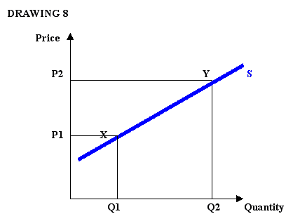
If demand is held constant, an increase in supply leads to a decreased price, while a decrease in supply leads to an increased price. This relationship can be illustrated in the form of a table called supply schedule and the data from the table may be given a diagrammatic representation in the form of a curve.

Read More

Demand Forecasting in Managerial Economics

One of the crucial aspects in which managerial economics differs from pure economic theory lies in the treatment of risk and uncertainty. Traditional economic theory assumes a risk-free world of certainty; but the real world business is full of all sorts of risk and uncertainty. A manager cannot, therefore, afford to ignore risk and uncertainty. The element of risk is associated with future which is indefinite and uncertain. To cope with future risk and uncertainty, the manager needs to predict the future event. The likely future event has to be given form and content in terms of projected course of variables, i.e. forecasting. Thus, business forecasting is an essential ingredient of corporate planning. Such forecasting enables the manager to minimize the element of risk and uncertainty. Demand forecasting is a specific type of business forecasting.

Concepts of Forecasting:

The manager can conceptualize the future in definite terms. If he is concerned with future event- its order, intensity and duration, he can predict the future. If he is concerned with the course of future variables- like demand, price or profit, he can project the future. Thus prediction and projection-both have reference to future; in fact, one supplements the other. Suppose, it is predicted that there will be inflation (event). To establish the nature of this event, one needs to consider the projected course of general price index (variable). Exactly in the same way, the predicted event of business recession has to be established with reference to the projected course of variables like sales, inventory etc.

Projection is of two types – forward and backward. It is a forward projection of data variables, which is named forecasting. By contrast, the backward projection of data may be named ‘back casting’, a tool used by the new economic historians. For practical managers concerned with futurology, what is relevant is forecasting, the forward projection of data, which supports the production of an event.

Thus, if a marketing manager fears demand recession, he must establish its basis in terms of trends in sales data; he can estimate such trends through extrapolation of his available sales data. This trend estimation is an exercise in forecasting.

Need for Demand Forecasting

Business managers, depending upon their functional area, need various forecasts. They need to forecast demand, supply, price, profit, costs and returns from investments.

The question may arise: Why have we chosen demand forecasting as a model? What is the use of demand forecasting?

The significance of demand or sales forecasting in the context of business policy decisions can hardly be overemphasized. Sales constitute the primary source of revenue for the corporate unit and reduction for sales gives rise to most of the costs incurred by the firm.

Demand forecasting is essential for a firm because it must plan its output to meet the forecasted demand according to the quantities demanded and the time at which these are demanded. The forecasting demand helps a firm to arrange for the supplies of the necessary inputs without any wastage of materials and time and also helps a firm to diversify its output to stabilize its income overtime.

The purpose of demand forecasting differs according to the type of forecasting.

(1) The purpose of the Short term forecasting:

It is difficult to define short run for a firm because its duration may differ according to the nature of the commodity. For a highly sophisticated automatic plant 3 months time may be considered as short run, while for another plant duration may extend to 6 months or one year. Time duration may be set for demand forecasting depending upon how frequent the fluctuations in demand are, short- term forecasting can be undertaken by affirm for the following purpose;

• Appropriate scheduling of production to avoid problems of over production and under- production.
• Proper management of inventories
• Evolving suitable price strategy to maintain consistent sales
• Formulating a suitable sales strategy in accordance with the changing pattern of demand and extent of competition among the firms.
• Forecasting financial requirements for the short period.

(2) The purpose of long- term forecasting:

The concept of demand forecasting is more relevant to the long-run that the short-run. It is comparatively easy to forecast the immediate future than to forecast the distant future. Fluctuations of a larger magnitude may take place in the distant future. In fast developing economy the duration may go up to 5 or 10 years, while in stagnant economy it may go up to 20 years. More over the time duration also depends upon the nature of the product for which demand forecasting is to be made. The purposes are;

• Planning for a new project, expansion and modernization of an existing unit, diversification and technological up gradation.
• Assessing long term financial needs. It takes time to raise financial resources.
• Arranging suitable manpower. It can help a firm to arrange for specialized labour force and personnel.
• Evolving a suitable strategy for changing pattern of consumption.

Read More

Steps in Demand Forecasting

Demand or sales forecasting is a scientific exercise. It has to go through a number of steps. At each step, you have to make critical considerations. Such considerations are categorically listed below:

1) Nature of forecast: To begin with, you should be clear about the uses of forecast data- how it is related to forward planning and corporate planning by the firm. Depending upon its use, you have to choose the type of forecasts: short-run or long-run, active or passive, conditional or non-conditional etc.

2) Nature of product: The next important consideration is the nature of product for which you are attempting a demand forecast. You have to examine carefully whether the product is consumer goods or producer goods, perishable or durable, final or intermediate demand, new demand or replacement demand type etc. A couple of examples may illustrate the importance of this factor. The demand for intermediate goods like basic chemicals is derived from the final demand for finished goods like detergents. While forecasting the demand for basic chemicals, it becomes essential to analyze the nature of demand for detergents. Promoting sales through advertising or price competition is much less important in the case of intermediate goods compared to final goods. The elasticity of demand for intermediate goods depends on their relative importance in the price of the final product.

Time factor is a crucial determinant in demand forecasting. Perishable commodities such as fresh vegetables and fruits can be sold over a limited period of time. Here skilful demand forecasting is needed to avoid waste. If there are storage facilities, then buyers can adjust their demand according to availability, price and income. The time taken for such adjustment varies from product to product. Goods of daily necessities that are bought more frequently will lead to quicker adjustments. Whereas in case of expensive equipment which is worn out and replaced after a long period of time, adaptation of demand will be spread over a longer duration of time.

3) Determinants of demand: Once you have identified the nature of product for which you are to build a forecast, your next task is to locate clearly the determinants of demand for the product. Depending on the nature of product and nature of forecasts, different determinants will assume different degree of importance in different demand functions.

In the preceding unit, you have been exposed to a number of price-income factors or determinants-own price, related price, own income-disposable and discretionary, related income, advertisement, price expectation etc. In addition, it is important to consider socio-psychological determinants, specially demographic, sociological and psychological factors affecting demand. Without considering these factors, long-run demand forecasting is not possible.

Such factors are particularly important for long-run active forecasts. The size of population, the age-composition, the location of household unit, the sex-composition-all these exercise influence on demand in. varying degrees. If more babies are born, more will be the demand for toys; if more youngsters marry, more will be the demand for furniture; if more old people survive, more will be the demand for sticks. In the same way buyers’ psychology-his need, social status, ego, demonstration effect etc. –also effect demand. While forecasting you cannot neglect these factors.

4) Analysis of factors &determinants: Identifying the determinants alone would not do, their analysis is also important for demand forecasting. In an analysis of statistical demand function, it is customary to classify the explanatory factors into (a) trend factors, which affect demand over long-run, (b) cyclical factors whose effects on demand are periodic in nature, (c) seasonal factors, which are a little more certain compared to cyclical factors, because there is some regularly with regard to their occurrence, and (d) random factors which create disturbance because they are erratic in nature; their operation and effects are not very orderly.

An analysis of factors is specially important depending upon whether it is the aggregate demand in the economy or the industry’s demand or the company’s demand or the consumers; demand which is being predicted. Also, for a long-run demand forecast, trend factors are important; but for a short-run demand forecast, cyclical and seasonal factors are important.

5) Choice of techniques: This is a very important step. You have to choose a particular technique from among various techniques of demand forecasting. Subsequently, you will be exposed to all such techniques, statistical or otherwise. You will find that different techniques may be appropriate for forecasting demand for different products depending upon their nature. In some cases, it may be possible to use more than one technique. However, the choice of technique has to be logical and appropriate; for it is a very critical choice. Much of the accuracy and relevance of the forecast data depends accuracy required, reference period of the forecast, complexity of the relationship postulated in the demand function, available time for forecasting exercise, size of cost budget for the forecast etc.

6) Testing accuracy: This is the final step in demand forecasting. There are various methods for testing statistical accuracy in a given forecast. Some of them are simple and inexpensive, others quite complex and difficult. This stating is needed to avoid/reduce the margin of error and thereby improve its validity for practical decision-making purpose. Subsequently you will be exposed briefly to some of these methods and their uses.

Read More

Techniques of Demand Forecasting

Broadly speaking, there are two approaches to demand forecasting- one is to obtain information about the likely purchase behavior of the buyer through collecting expert’s opinion or by conducting interviews with consumers, the other is to use past experience as a guide through a set of statistical techniques. Both these methods rely on varying degrees of judgment. The first method is usually found suitable for short-term forecasting, the latter for long-term forecasting. There are specific techniques which fall under each of these broad methods.

Simple Survey Method:

For forecasting the demand for existing product, such survey methods are often employed. In this set of methods, we may undertake the following exercise.

1) Experts Opinion Poll: In this method, the experts on the particular product whose demand is under study are requested to give their ‘opinion’ or ‘feel’ about the product. These experts, dealing in the same or similar product, are able to predict the likely sales of a given product in future periods under different conditions based on their experience. If the number of such experts is large and their experience-based reactions are different, then an average-simple or weighted –is found to lead to unique forecasts. Sometimes this method is also called the ‘hunch method’ but it replaces analysis by opinions and it can thus turn out to be highly subjective in nature.

2) Reasoned Opinion-Delphi Technique: This is a variant of the opinion poll method. Here is an attempt to arrive at a consensus in an uncertain area by questioning a group of experts repeatedly until the responses appear to converge along a single line. The participants are supplied with responses to previous questions (including seasonings from others in the group by a coordinator or a leader or operator of some sort). Such feedback may result in an expert revising his earlier opinion. This may lead to a narrowing down of the divergent views (of the experts) expressed earlier. The Delphi Techniques, followed by the Greeks earlier, thus generates “reasoned opinion” in place of “unstructured opinion”; but this is still a poor proxy for market behavior of economic variables.

3) Consumers Survey- Complete Enumeration Method: Under this, the forecaster undertakes a complete survey of all consumers whose demand he intends to forecast, Once this information is collected, the sales forecasts are obtained by simply adding the probable demands of all consumers. The principle merit of this method is that the forecaster does not introduce any bias or value judgment of his own. He simply records the data and aggregates. But it is a very tedious and cumbersome process; it is not feasible where a large number of consumers are involved. Moreover if the data are wrongly recorded, this method will be totally useless.

4) Consumer Survey-Sample Survey Method: Under this method, the forecaster selects a few consuming units out of the relevant population and then collects data on their probable demands for the product during the forecast period. The total demand of sample units is finally blown up to generate the total demand forecast. Compared to the former survey, this method is less tedious and less costly, and subject to less data error; but the choice of sample is very critical. If the sample is properly chosen, then it will yield dependable results; otherwise there may be sampling error. The sampling error can decrease with every increase in sample size

5) End-user Method of Consumers Survey: Under this method, the sales of a product are projected through a survey of its end-users. A product is used for final consumption or as an intermediate product in the production of other goods in the domestic market, or it may be exported as well as imported. The demands for final consumption and exports net of imports are estimated through some other forecasting method, and its demand for intermediate use is estimated through a survey of its user industries.

Complex Statistical Methods:

We shall now move from simple to complex set of methods of demand forecasting. Such methods are taken usually from statistics. As such, you may be quite familiar with some the statistical tools and techniques, as a part of quantitative methods for business decisions.

(1) Time series analysis or trend method: Under this method, the time series data on the under forecast are used to fit a trend line or curve either graphically or through statistical method of Least Squares. The trend line is worked out by fitting a trend equation to time series data with the aid of an estimation method. The trend equation could take either a linear or any kind of non-linear form. The trend method outlined above often yields a dependable forecast. The advantage in this method is that it does not require the formal knowledge of economic theory and the market, it only needs the time series data. The only limitation in this method is that it assumes that the past is repeated in future. Also, it is an appropriate method for long-run forecasts, but inappropriate for short-run forecasts. Sometimes the time series analysis may not reveal a significant trend of any kind. In that case, the moving average method or exponentially weighted moving average method is used to smoothen the series.

(2) Barometric Techniques or Lead-Lag indicators method: This consists in discovering a set of series of some variables which exhibit a close association in their movement over a period or time.

For example, it shows the movement of agricultural income (AY series) and the sale of tractors (ST series). The movement of AY is similar to that of ST, but the movement in ST takes place after a year’s time lag compared to the movement in AY. Thus if one knows the direction of the movement in agriculture income (AY), one can predict the direction of movement of tractors’ sale (ST) for the next year. Thus agricultural income (AY) may be used as a barometer (a leading indicator) to help the short-term forecast for the sale of tractors.

Generally, this barometric method has been used in some of the developed countries for predicting business cycles situation. For this purpose, some countries construct what are known as ‘diffusion indices’ by combining the movement of a number of leading series in the economy so that turning points in business activity could be discovered well in advance. Some of the limitations of this method may be noted however. The leading indicator method does not tell you anything about the magnitude of the change that can be expected in the lagging series, but only the direction of change. Also, the lead period itself may change overtime. Through our estimation we may find out the best-fitted lag period on the past data, but the same may not be true for the future. Finally, it may not be always possible to find out the leading, lagging or coincident indicators of the variable for which a demand forecast is being attempted.

3) Correlation and Regression: These involve the use of econometric methods to determine the nature and degree of association between/among a set of variables. Econometrics, you may recall, is the use of economic theory, statistical analysis and mathematical functions to determine the relationship between a dependent variable (say, sales) and one or more independent variables (like price, income, advertisement etc.). The relationship may be expressed in the form of a demand function, as we have seen earlier. Such relationships, based on past data can be used for forecasting. The analysis can be carried with varying degrees of complexity. Here we shall not get into the methods of finding out ‘correlation coefficient’ or ‘regression equation’; you must have covered those statistical techniques as a part of quantitative methods. Similarly, we shall not go into the question of economic theory. We shall concentrate simply on the use of these econometric techniques in forecasting.

We are on the realm of multiple regression and multiple correlation. The form of the equation may be:

D_X = a + b₁ A + b₂P_X + b₃P_y

You know that the regression coefficients b₁, b₂, b₃ and b₄ are the components of relevant elasticity of demand. For example, b₁ is a component of price elasticity of demand. The reflect the direction as well as proportion of change in demand for x as a result of a change in any of its explanatory variables. For example, b₂<>X

and P_X are inversely related; b₄ > 0 suggest that x and y are substitutes; b₃ > 0 suggest that x is a normal commodity with commodity with positive income-effect.

Given the estimated value of and b_i, you may forecast the expected sales (D_X), if you know the future values of explanatory variables like own price (P_X), related price (P_y), income (B) and advertisement (A). Lastly, you may also recall that the statistics R2 (Co-efficient of determination) gives the measure of goodness of fit. The closer it is to unity, the better is the fit, and that way you get a more reliable forecast.

The principle advantage of this method is that it is prescriptive as well descriptive. That is, besides generating demand forecast, it explains why the demand is what it is. In other words, this technique has got both explanatory and predictive value. The regression method is neither mechanistic like the trend method nor subjective like the opinion poll method. In this method of forecasting, you may use not only time-series data but also cross section data. The only precaution you need to take is that data analysis should be based on the logic of economic theory.

(4) Simultaneous Equations Method: Here is a very sophisticated method of forecasting. It is also known as the ‘complete system approach’ or ‘econometric model building’. In your earlier units, we have made reference to such econometric models. Presently we do not intend to get into the details of this method because it is a subject by itself. Moreover, this method is normally used in macro-level forecasting for the economy as a whole; in this course, our focus is limited to micro elements only. Of course, you, as corporate managers, should know the basic elements in such an approach.

The method is indeed very complicated. However, in the days of computer, when package programmes are available, this method can be used easily to derive meaningful forecasts. The principle advantage in this method is that the forecaster needs to estimate the future values of only the exogenous variables unlike the regression method where he has to predict the future values of all, endogenous and exogenous variables affecting the variable under forecast. The values of exogenous variables are easier to predict than those of the endogenous variables. However, such econometric models have limitations, similar to that of regression method.

Read More

Foreign Trade Policy of India

Foreign Trade Policy of India for the time period 27th August 2009 - 31st March 2014.
to see more download this PDF:

http://www.mediafire.com/?8zpa166ni108epp

Read More